Steel Surface Defect Diagnostics Using Deep Convolutional Neural Network and Class Activation Map


1
Department of Mechanical Engineering, Pohang University of Science and Technology (POSTECH), Pohang 37673, Korea
2
Department of System Dynamics, Korea Institute of Machinery and Materials, Daejeon 34103, Korea
*
Author to whom correspondence should be addressed.
Appl. Sci. 2019, 9(24), 5449; https://doi.org/10.3390/app9245449
Submission received: 14 November 2019
/
Revised: 5 December 2019
/
Accepted: 6 December 2019
/
Published: 12 December 2019
(This article belongs to the Special Issue Selected Papers from the ICMR 2019)
Abstract
:Steel defect diagnostics is considerably important for a steel-manufacturing industry as it is strongly related to the product quality and production efficiency. Product quality control suffers from a real-time diagnostic capability since it is less-automatic and is not reliable in detecting steel surface defects. In this study, we propose a relatively new approach for diagnosing steel defects using a deep structured neural network, e.g., convolutional neural network (CNN) with class activation maps. Rather than using a simple deep learning algorithm for the classification task, we extend the CNN diagnostic model for being used to analyze the localized defect regions within the images to support a real-time visual decision-making process. Based on the experimental results, the proposed approach achieves a near-perfect detection performance at 99.44% and 0.99 concerning the accuracy and F-1 score metric, respectively. The results are better than other shallow machine learning algorithms, i.e., support vector machine and logistic regression under the same validation technique.
1. Introduction
Quality inspection and control in the steel-manufacturing industry have been a critical issue for assuring the product quality and increasing its productivity. As a steel defect is deemed to be one of the main causes of the production cost increase, monitoring the quality of steel products is inevitable during the manufacturing process [1]. The defects can be attributed to various factors, e.g., operational conditions and facilities [2,3]. For an immediate response and control about the flaws, detecting steel defects should be preceded to analyze the failure causes. To this end, a sophisticated diagnostic model is required to detect the failures properly and to enhance the capability of quality control.
In particular, a vision-based diagnostics system for detecting the steel surface defects has received considerable attention. The traditional human inspection system has several disadvantages such as a less-automatic and time-consuming procedure [4,5]. An image-based system, on the other hand, is developed to enable more elaborate, rapid and automatic inspection than the existing methods [6]. Furthermore, it is widely known that the surface defect accounts for more than 90% of entire defects in steel products, e.g., plate and strip [7]. Defects on the steel surface, e.g., scratches, patches, and inclusions exert maleficent influence on material properties, i.e., fatigue strength and corrosion resistance, as well as the appearance [8]. Likewise, the development of a visual inspection system for identifying steel surface defects should be conducted to secure the reliability of the process and the product.
Over recent years, a variety of research-based on machine learning and deep learning techniques have been conducted to establish defect diagnostics model of the steel surface with machine-vision, showing feasible performance for an automatic inspection system. For example, Jia, et al. [9] suggest a real-time surface defect detection method using a support vector machine (SVM) classifier, demonstrating the prediction accuracy of 85%. Batsuuri, et al. [10] present feature extraction and region-based defect detection method via scale-invariant feature transform (SIFT) to enhance the accuracy with limited samples. Especially, convolutional neural network (CNN) based detection methods are widely utilized as a way of the end-to-end framework for image processing, feature learning, and classification, achieving remarkable improvement in diagnosis performance [11,12,13].
To take advantage of the deep learning framework, many researches have been conducted, in particular, application with CNN. A max-pooling CNN for steel defect classification is introduced in [14]. A max-pooling CNN approach is used for classifying seven different types of steel defects from a real production line. The proposed network uses supervised feature extraction directly from the steel images so that it enables to work without prior knowledge. The optimal model of the proposed one attains an error rate of 7%. Work in [15] considers an image-based method for detecting corner cracks of steel billet surface using wavelet reconstruction to reduce the influence of scales. However, its processing time requires a more considerable cost than a deep neural network-based method due to the computation of the wavelet decomposition and reconstruction.
An ensemble of support vector machine (SVM) classifiers for steel surface defects with a small sample set is introduced in [16]. Some features are obtained from a set of extractors techniques for being used as the inputs of an SVM ensemble, where a combiner, called Bayes kernel is employed to fuse the results from SVM classifiers. Chen, et al. [7] suggest an integrated framework with CNN and naïve Bayes data fusion scheme for detecting cracks in nuclear power plants. This work utilizes a data fusion strategy so that spatiotemporal features of the cracks in videos are efficiently used, showing improved achievement of 98.3% hit rate toward the traditional inspection system of a nuclear power plant. More recently, Gao, et al. [17] propose a semi-supervised approach for steel surface defect recognition based on CNN. The method has better performances with 17.53% improvement compared to the baselines. Also, it has been applied in a real-world detection scenario with a limited labeled dataset.
Although several studies have been conducted to enhance the defect detection performance in the steel surface, there are still challenging issues for practical use, which motivates this study. Firstly, the optimization of a deep neural network-based model should be conducted. Tuning the hyper-parameters and building the optimized architectural structure should be carried out to maximize the classification performance for detecting the steel surface defects. Besides, training the network and an over fitting problem could be a practical issue while operating for both observed and unobserved data. Secondly, decisions made by deep learning algorithms should be interpretable. Connections between input and output of a deep neural network-based model could not be described using specific mathematical analyses or mapping functions. When the defect is detected during the process, the explanation should be given to demonstrate the basis of the decision-making of a black-box model.
Imbued by the above-mentioned challenges, this paper proposes a convolutional neural network (CNN) based detection method for improving vision-based diagnostics model and enhancing its explainability while classifying steel surface defects. The CNN classification model is developed to learn high-dimensional characteristics of spatial information, being developed to discriminate among 6 different kinds of surface defects, i.e., rolled-in scale, patches, crazing, pitted surface, inclusion, and scratches. Furthermore, class activation map (CAM) is localized to describe the most significant parts from the images, providing as an interpreter of the results. To validate our proposed method, the performance resulted from the proposed model is compared with conventional machine learning-based classification algorithms, i.e., support vector machine (SVM) and logistic regression.
2. Background
In this section, we shortly explain the feature extraction methods in image processing which are used for machine learning algorithms, followed by fundamentals of convolutional neural network (CNN) and class activation map (CAM).
2.1. Feature Extraction Methods
2.1.1. Gray Level Co-Occurrence Matrix
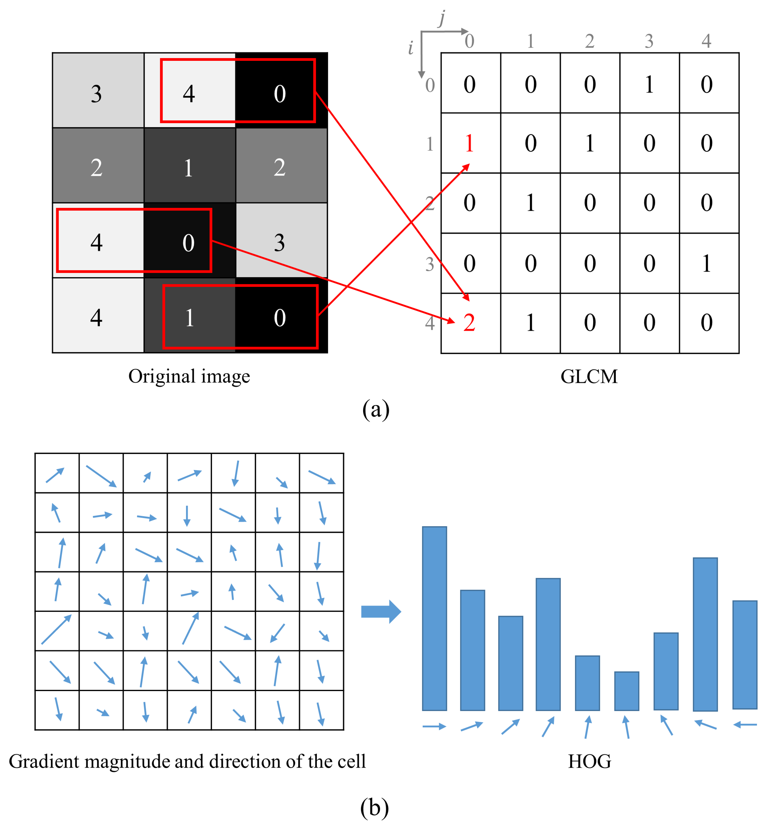
Gray level co-occurrence matrix (GLCM), proposed by Haralick et al. [18], is a two-dimensional matrix that contains statistical information about the texture of the single-channel image. While the images are generally comprised of three different layers, i.e., red, green and blue, GLCM utilizes a single level of the gray image. Briefly speaking, texture analysis could be carried out while statistically considering the spatial relationship from the GLCMs. The matrix is generated by the pixel values in the image, calculating the frequency sum of adjacent pixel pairs in a particular region. Owing to its advantages of extracting the features from the images, it has been utilized to the image analysis tasks in a variety of fields, e.g., medical, material and manufacturing [19,20,21].
A method for calculating the GLCM is schematically described in Figure 1a. In a grey-scale original image, the co-occurrence of the paired pixel values which are represented as the numbers in the figure is counted at a given offset. By and large, the offset can be varied over degrees, i.e., horizontal, vertical and diagonal. The coordinates of the GLCM, i and j, are determined based on the previous pixel values from the gray-level image, while the frequency sum of the counts is calculated via the intensity values from the original image and assigned to the GLCM as corresponding to the coordinates. Since the pixel value of the original image ranges between 0 and 255, basically 256 × 256 of the GLCM can be produced. Finally, several second-order statistical features for the texture analysis, i.e., angular second moment (ASM), contrast, entropy, and homogeneity, are defined as follows [18,22].
2.1.2. Histogram of Oriented Gradients
Histogram of oriented gradients (HOG) is the gradient-based feature descriptor for extracting the image features, generating the histograms based on gradient magnitude and direction [23]. The gradient magnitude and direction can be calculated via pixel values within an image, while edges and shapes in the image can be efficiently described by the gradient-based histograms. On account of being able to represent the image appearance, the HOG has been developed to outperform visual object detection analysis [24,25]. The gradient magnitude g and the gradient direction can be calculated using the gradients in two directions as follows.
The histogram of oriented gradients is formed as shown in Figure 1b. The gradient magnitudes and directions are calculated within the image, where the directions are the angles between 0° to 180°. Those gradient directions compose user-specified bins of the histogram as a way of orientation binning, while the magnitudes are allocated to the bins. A series of the processes are conducted in all divided regions from the entire image, which are called cells. Accordingly, the gradient amplitudes of the bins locally provide feature representation for difference among the pixel intensity values and its orientation from the histograms.
2.2. Fundamentals of CNN and CAM
A convolutional neural network (CNN) is a type of deep neural network using successive operations across a variety of layers, which is specified to deal with a two-dimensional image. CNN, firstly introduced in [26], is known to be a successful neural network algorithm for image processing and recognition. The CNN architecture is typically made up of two main stages, i.e., feature extraction and classification, while it is learned to describe spatial information of the images across the layers. Extracted feature representations are fed into the latter part of the architecture, where the model draws a probability for belonging to a certain class. Likewise, weights and biases of the model are optimized by training the neural network via the back propagation algorithm.
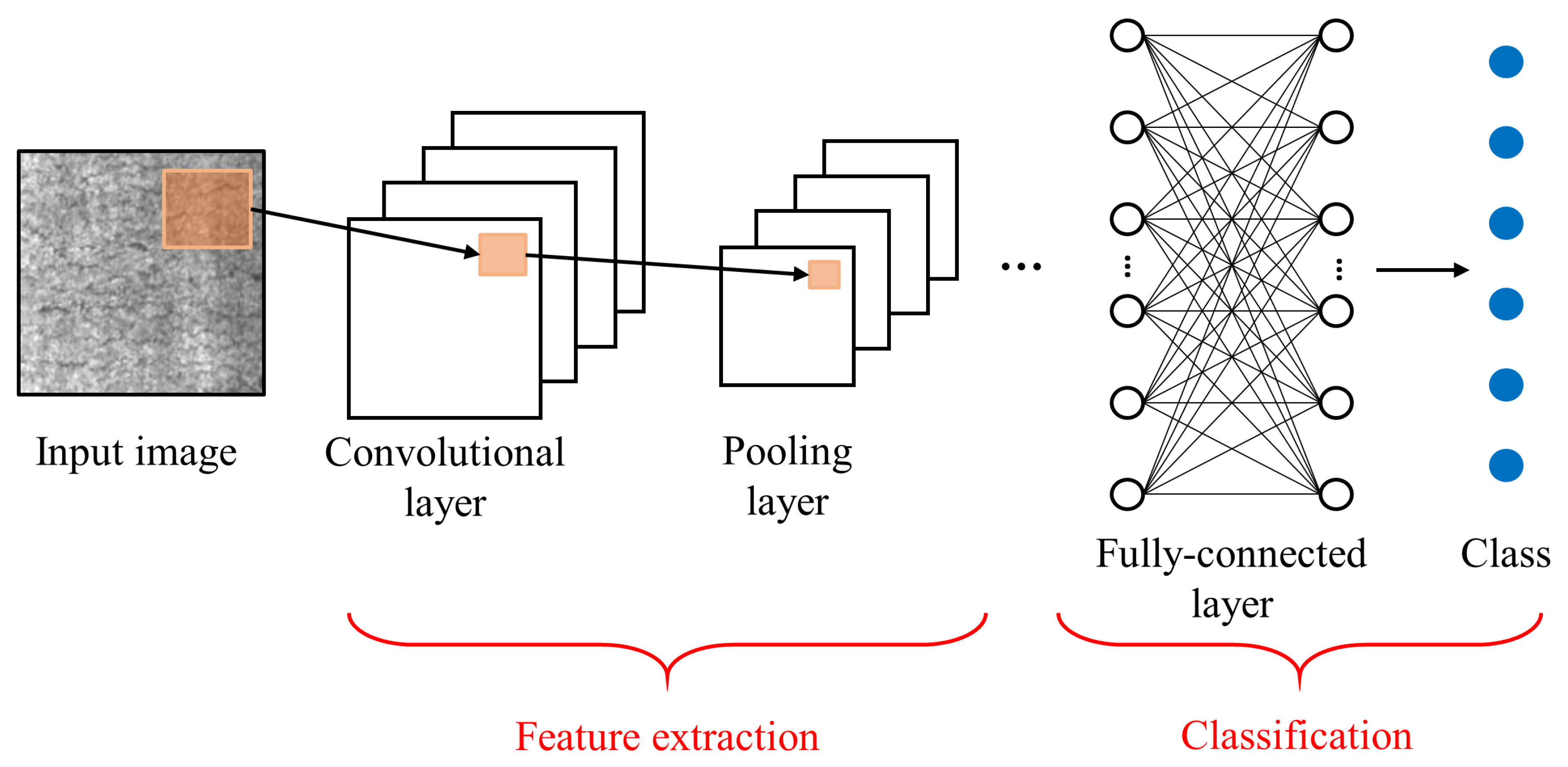
There are conventionally three different types of layers in the CNN architecture, i.e., convolutional, pooling and fully-connected layer (see Figure 2). The convolutional layer utilizes convolution operation to extract spatial features of the image, herein feature maps are computed by utilizing element-wise multiplication between the input image and the operator called kernel or filter. The pooling layer is carried out as a sub-sampling technique, followed by the convolution layer. It is aimed at downsizing the convoluted feature maps to reduce the number of trainable parameters, as well as to improve invariance for shift and distortion. A typical pooling method, i.e., max pooling, is used by taking the highest-value tensors from each certain region in the feature maps. Lastly, the fully-connected layer utilizes intensive features created through two types of layers, i.e., convolutional and pooling layers, for categorizing the input images into classes.
A class activation map (CAM) method can be deployed to the CNN architecture using global average pooling for enhancing the visual explanation of the deep neural network-based model [27]. The attention map is activated in a way of class-discriminative regions, highlighting the significance within the image for the classification. Through the supplementary analysis on which region the CNN model concentrates for classification, it provides interpretability to judge the black-box model, besides the insights can be obtained to establish the CNN model with more enhanced performance. The CAM can be obtained by taking a linear sum of the feature maps that passes through the last convolutional and pooling layer as follows.
where is the class activation map for a certain class c. denotes the weight value corresponding to c for unit, while represents the feature map at spatial location .
3. Proposed Method
In this section, we briefly explain the outline of the research, followed by details of deep learning-based proposed architecture using a convolutional neural network and class activation map, as well as parametric measures used in the experiment.
3.1. Research Outline
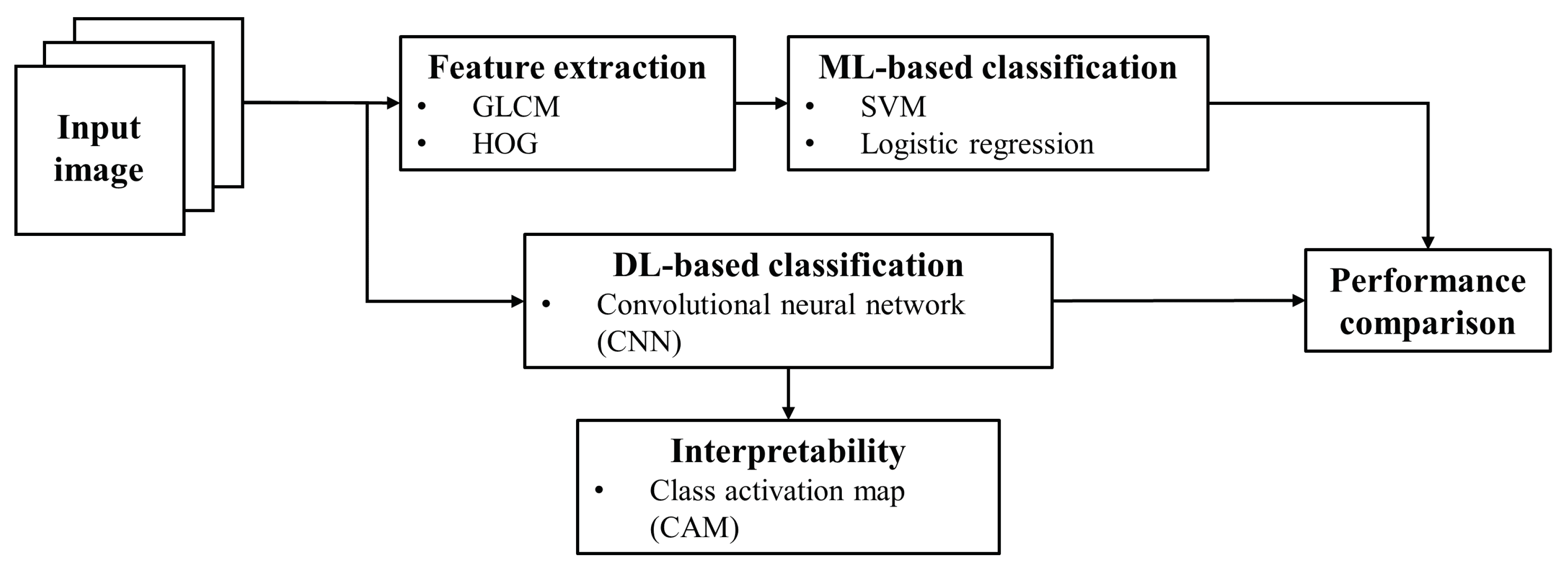
In this study, several approaches are conducted to validate the improved reliability of the proposed method for steel surface defects diagnostics. The approaches can be divided into two main strategies as shown in Figure 3. First of all, the machine learning (ML) based classification model is adopted for a comparative study with a deep neural network-based diagnostics model. Input images are preprocessed as statistical texture features, i.e., ASM, contrast, entropy and homogeneity, and gradient-based histograms from GLCM and HOG, respectively, where the extracted features are fed into to the ML-based model, i.e., SVM and logistic regression for categorizing into a particular class. Secondly, as a way of deep learning (DL) algorithm, the CNN model is constructed as an end-to-end framework of feature learning and classification process, utilizing the raw input image as it is. The performances of ML and DL based approaches are compared and evaluated in terms of accuracy and F1-score metric. In particular, the DL-based CNN model includes a global average pooling (GAP) operation for producing attention maps, which can enrich the interpretability of the model. Class activation maps are described to visualize the most salient regions for decision-making of the CNN diagnostics model.
3.2. Network Architecture
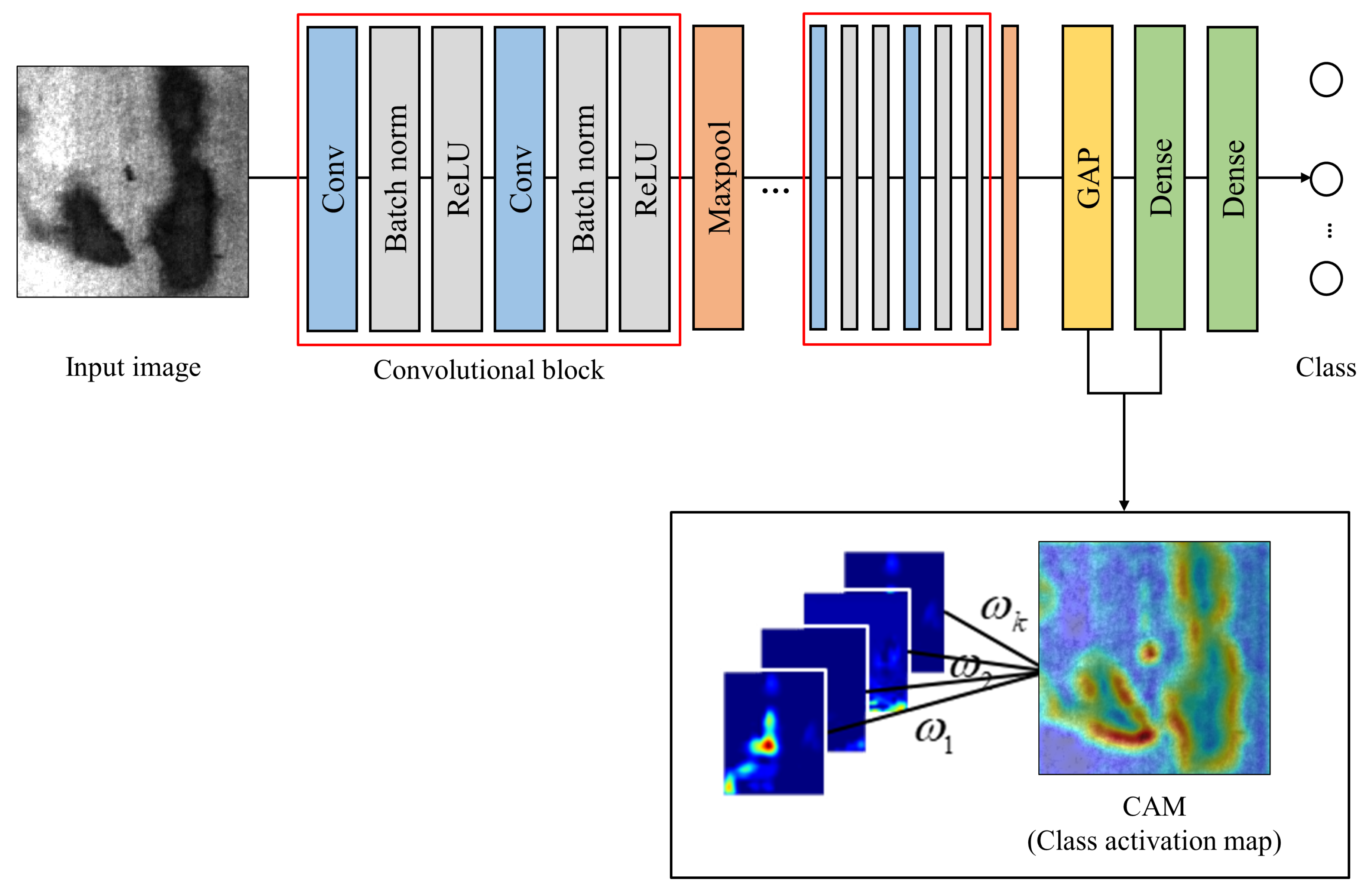
The descriptions of the proposed CNN with CAM architecture are presented in Figure 4 and Table 1. Inspired by VGG-Net introduced by Karen Simonyan et al. [28], we built a VGG-like CNN model that has a total of 17 layers with different types of operations, i.e., convolution, max pooling, global average pooling and dense. In particular, the model is comprised of five convolutional blocks, where each convolutional block refers to a combination of two consecutive convolutional layers and a max-pooling layer. Two convolutional layers in the block share the same kernel size of 3 × 3 and the number of channels. It is proved that taking advantage of the small size of the filters makes receptive fields more simple, where it is possible to increase the depth of the architecture [28]. Also, we utilized batch normalization and rectified linear unit (ReLU), which are appended between every convolutional layer. The former is used to normalize each training mini-batch for resolving overfitting problems as a regularizer [29], while the latter serves as a nonlinear activation function. Besides, the global average pooling (GAP) is taken into account to visualize activation maps for understanding the discriminative results of the proposed network. Finally, the latter part of the network is fully connected layers and an output layer with six neurons, corresponding to the number of steel surface defects categories.
3.3. Parametric Measures
The performance of the classification model can be measured in several ways. In our experiments, accuracy and F1-score are used to evaluate the performance for classifying the steel surface defects. The accuracy is one of the most common evaluation measures, which denotes the ratio of the number of properly classified samples to one of the entire testing samples. The accuracy metric can be defined as follows.
where TP, TN, FP, and FN are the abbreviations for true positive, true negative, false positive and false negative, respectively. Those components can be calculated with a confusion matrix that indicates a table of classified results between actual and predicted classes. Besides, F1-score is adopted in this study to further investigate the performance when the testing data set is unbalanced. Unless the testing data set is completely divided in a way of stratified sampling, it would not be enough to investigate only the accuracy metric. It is a harmonic mean value between precision and recall metric, which can be determined as follows.
4. Experimental Results and Discussion
4.1. Data Description
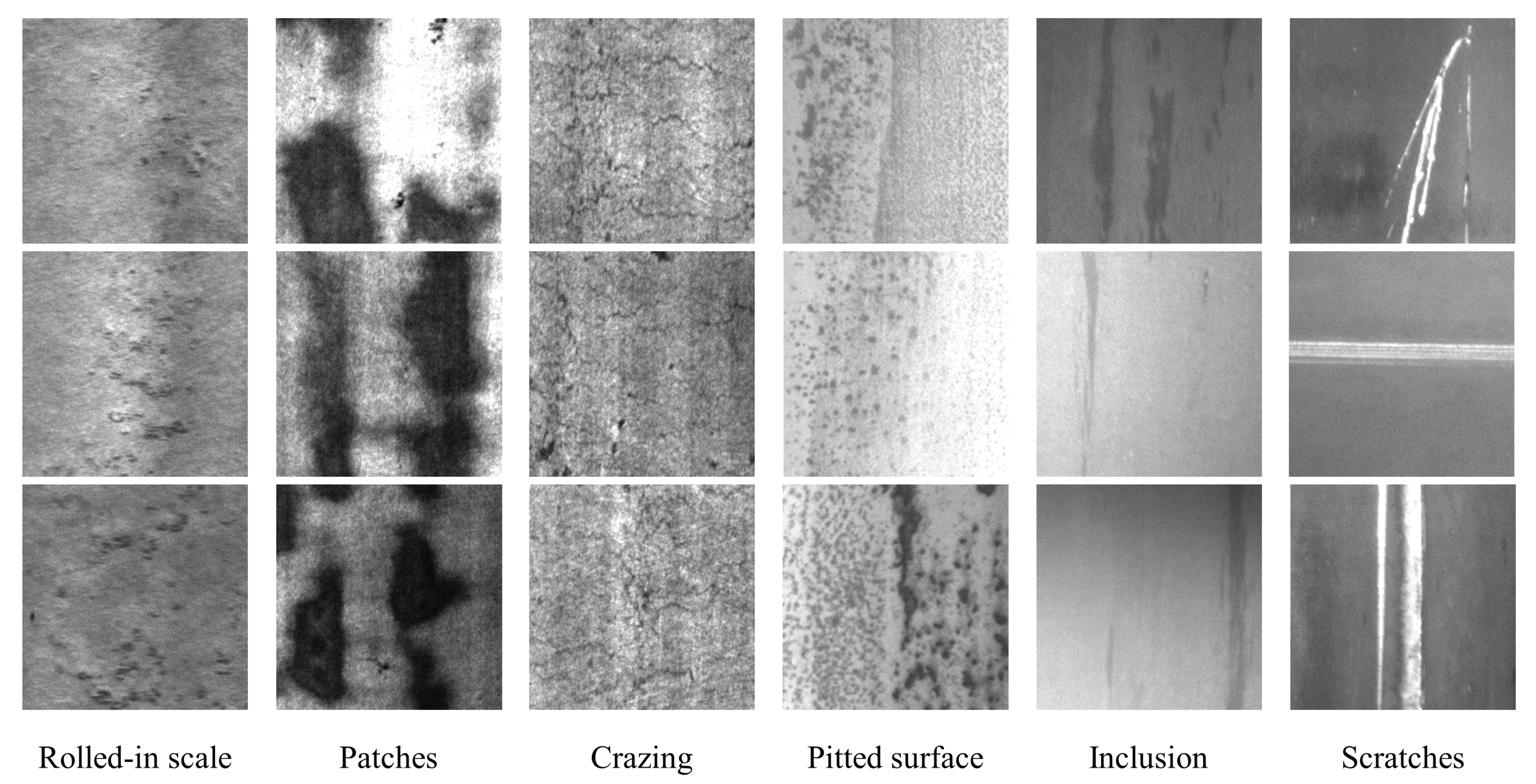
Provided by Song and Yan [8], the NEU data set is utilized to establish a steel surface defect diagnostics model. The data set is made up of six different kinds of defect cases, i.e., rolled-in scale, patches, crazing, pitted surface, inclusion, and scratches. Figure 5 visualizes several example images of the steel surface defect cases used in the experiment. Besides, as described in Table 2, each class has 300 samples, where each sample is an image with a dimension of 200 × 200. In the experiment, the entire data set is randomly split into training, validation and testing data set, where 70% of the whole images are used as a training set whilst 20% and 10% of them are, respectively, used as testing and validation set. The main challenging issue of the described data set is confusing spatial characteristics of the images. In some cases, it is difficult to identify spatial information as it sporadically appears in different aspects of the images. For example, patterns in the scratches differ from horizontal to vertical stripes. Also, the gray-scale of the images frequently varies due to the illumination effect [8].
4.2. Performance of Steel Surface Defect Classification
Classification accuracy and F1-scores for identifying the steel surface defects are measured among the classifiers, which are generally divided into two categories according to the type of algorithms, i.e., machine learning (ML) and deep learning (DL) based method. The former method is used to train shallow classification models, i.e., SVM and logistic regression, while the latter one is based on a convolutional neural network with a class activation map. Each model is trained using an optimized hyper-parameters setting of random search method, where 5-fold cross-validation is carried out. Early stopping strategy is also utilized to avoid overfitting problem with a separate validation set while monitoring the training process. Likewise, the performance of the proposed CNN model is evaluated and compared with the trained ML-based models for a comparative purpose.
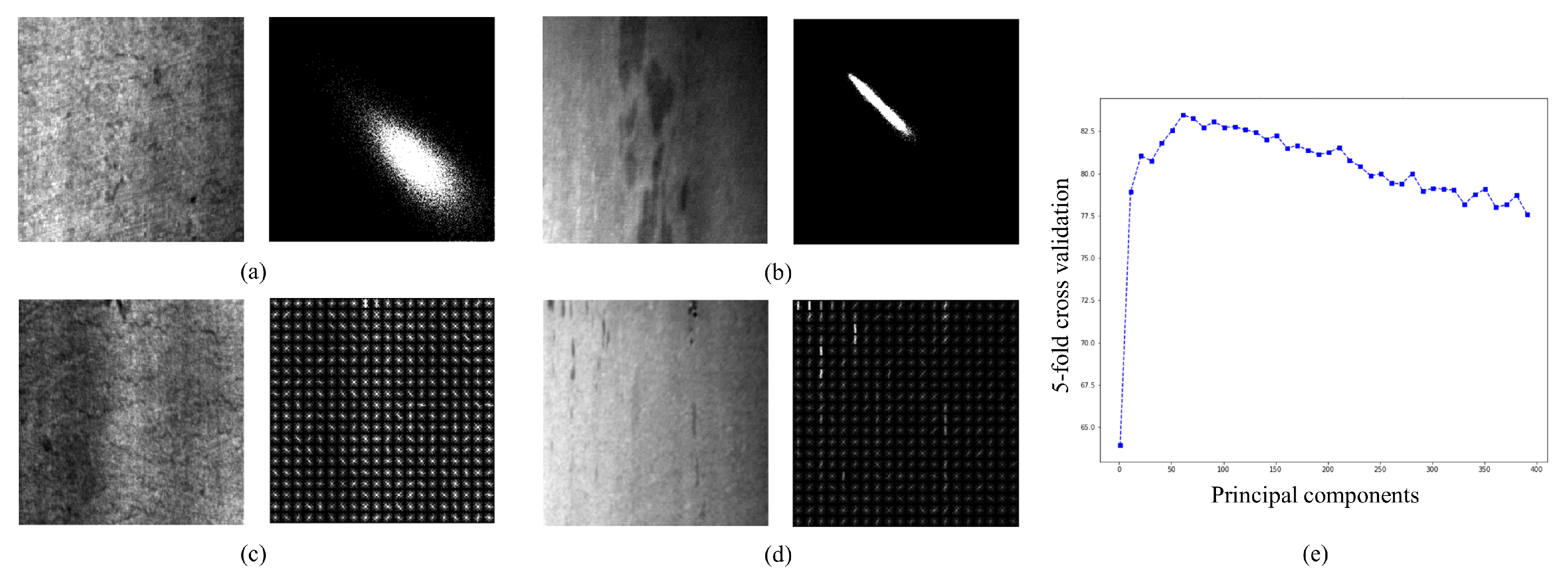
Unlike the DL based models using the end-to-end learning process, a manual feature extraction procedure is beforehand required for the input images of ML algorithms. As previously mentioned in Section 3, GLCM and HOG are deployed to extract numeric feature representations. Figure 6 illustrates examples of extracted features from images. The examples denote both calculated features in crazing and inclusion cases, representing visually distinguishable patterns of textural and gradient-based characteristics. While four kinds of statistical texture features, i.e., ASM, contrast, entropy, and homogeneity, are drawn via the GLCM method, particularly the gradient-based histograms are made up of thousands of gradient amplitudes in the consequence of nine direction bins in each cell. Instead of using the entire histograms extracted from HOG, the optimal 60 components which indicate the highest average accuracy from 5-fold cross-validation are determined via principal component analysis (PCA) (see Figure 6e).
The classification performance of traditional ML algorithms, i.e., SVM and logistic regression, are described in Table 3. Generally, it is shown that GLCM has performed better than HOG concerning accuracy and F1-score in both classifiers. It is also proved that features combination model (denoted as GLCM+HOG) outperforms the model with a single feature, given the fact that concatenated two kinds of features are expected to consider not only texture but histogram distribution, thus it is likely to earn more rich representations of the features. In ML-based models, the SVM with GLCM and HOG shows the best performance of 92.22% accuracy and 0.91 F1-score, whereas the one with HOG yields the worst accuracy and F1-score by 78.61% and 0.77, respectively.
Without the manual design of the features, the proposed CNN architecture is established to conduct feature learning and classification throughout the network. The performance of CNN is described in Table 3. The proposed CNN model with hyper-parameter optimization attains a remarkable performance in both accuracy and F1-score, compared to the ML-based models. It is observed that the testing accuracy of CNN is 99.44% and the F1-score is nearly close to 1.00, especially showing approximately 8% improved accuracy over the traditional ones. Herein, a randomly split testing set has 360 images, which are 20% of the whole data set.
We compare our proposed model with several previous works that propose steel surface defect diagnostics using the same data set (see Table 4). Some of them have used machine learning-based approaches and manual feature extraction, called the adjacent evaluation completed local binary patterns (AECLBPs) [8] and a combination of multiple extractor techniques [16]. Other approaches such as [12,17] have utilized CNN as the way of end-to-end learning framework. Both machine learning-based studies have shown unfeasible results in terms of accuracy at 98.93% and 96.39%, respectively. Meanwhile, it is evidenced that our proposed CNN architectural model achieves more improved testing accuracy of 99.44%, compared to other deep learning-based algorithms, i.e., CNN [12,17].
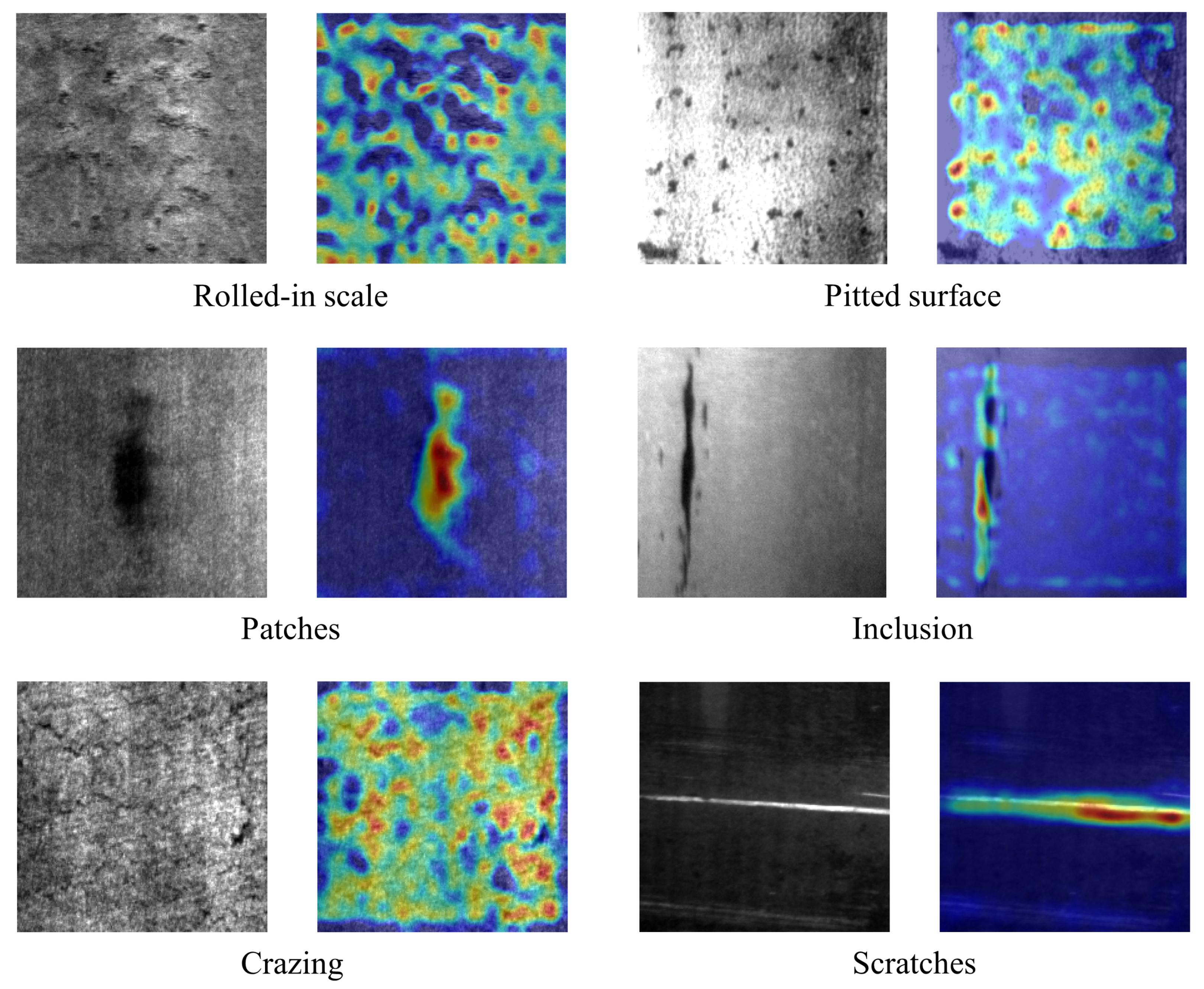
We are also interested to observe the interpretability of deep learning-based methods, where the class activation maps (CAMs) can be drawn out from the proposed CNN diagnostics model. To analyze the localized regions for decision-making, the attention maps are described in Figure 7. Each pair of figures presents an original image of steel surface defect and a localization map in a particular class, retrieved from our proposed model. Depending upon the category, it is observed that each attention map differently localizes in its certain way, while more attention goes from blue to red region, the more it emphasizes. It is also found that there are two main types of attention, i.e., global and local attention. For example, classes that have locally affected parts, i.e., patches, inclusion, and scratches, tend to activate sub-regional features such as spots and stripes. On the other hand, for globally characterized categories, i.e., rolled-in-scale, pitted surface, and crazing, the map is more likely to be highlighted in a wide region, as they have global scattered patterns, e.g., speckles, bumps, and cracks. Consequently, the most salient part from the images for classification is appropriately described in the CAM, which enables interaction between human decision and black-box based deep learning approach. To sum up, by constructing the global average pooling layer in the proposed architecture, the class activation map could be described for enhancing the interpretability of the proposed network, which lacks in the prior studies.
5. Conclusions
In this paper, we proposed a steel surface defect detection based on a convolutional neural network with a class activation map. It was clear that the proposed model outperformed other shallow machine learning algorithms, i.e., support vector machine and logistic regression in terms of accuracy and F-1 metrics. Our detection model was comparable in comparison with similar previous deep learning-based models, e.g., CNN and PLCNN concerning accuracy metric. Besides, the explainability of the deep learning model was also discussed by providing a localized region within the steel defect image to support decision making. This ability bridged significantly between human-expert decisions and the black-box model of deep learning. Among the possible ways to extend this study, future work might consider other large-scale steel defect datasets and more precisely, the use of an advanced technique that could classify multiple defect categories within an image would be desirable.
Author Contributions
Conceptualization, S.Y.L.; methodology, S.Y.L. and B.A.T.; writing—original draft preparation, S.Y.L. and B.A.T.; writing—review and editing, B.A.T.; supervision, S.L.; funding acquisition, S.L. and S.J.M.
Funding
This work was supported in part by the Technology Innovation Program of the Ministry of Trade, Industry and Energy (MOTIE) under Grant 10080729, in part by the Korea Institute for Advancement of Technology (KIAT) grant funded by the Korea Government (N0008691, The Competency Development Program for Industry Specialist) and in part by the High-Potential Individuals Global Training Program of Institute for Information and Communications Technology Planning Evaluation (IITP) under Grant 2019-0-01589.
Conflicts of Interest
The authors declare no conflict of interest.
References
- Song, G.W.; Tama, B.A.; Park, J.; Hwang, J.Y.; Bang, J.; Park, S.J.; Lee, S. Temperature Control Optimization in a Steel-Making Continuous Casting Process Using Multimodal Deep Learning Approach. Steel Res. Int. 2019, 90, 1900321. [Google Scholar] [CrossRef]
- Luo, Q.; He, Y. A cost-effective and automatic surface defect inspection system for hot-rolled flat steel. Robot. Comput.-Integr. Manuf. 2016, 38, 16–30. [Google Scholar] [CrossRef]
- Ghorai, S.; Mukherjee, A.; Gangadaran, M.; Dutta, P.K. Automatic defect detection on hot-rolled flat steel products. IEEE Trans. Instrum. Meas. 2012, 62, 612–621. [Google Scholar] [CrossRef]
- He, Y.; Song, K.; Meng, Q.; Yan, Y. An End-to-end Steel Surface Defect Detection Approach via Fusing Multiple Hierarchical Features. IEEE Trans. Instrum. Meas. 2019. [Google Scholar] [CrossRef]
- Choi, W.; Huh, H.; Tama, B.A.; Park, G.; Lee, S. A Neural Network Model for Material Degradation Detection and Diagnosis Using Microscopic Images. IEEE Access 2019, 7, 92151–92160. [Google Scholar] [CrossRef]
- Liu, K.; Wang, H.; Chen, H.; Qu, E.; Tian, Y.; Sun, H. Steel surface defect detection using a new Haar–Weibull-variance model in unsupervised manner. IEEE Trans. Instrum. Meas. 2017, 66, 2585–2596. [Google Scholar] [CrossRef]
- Chen, W.; Gao, Y.; Gao, L.; Li, X. A New Ensemble Approach based on Deep Convolutional Neural Networks for Steel Surface Defect classification. Procedia CIRP 2018, 72, 1069–1072. [Google Scholar] [CrossRef]
- Song, K.; Yan, Y. A noise robust method based on completed local binary patterns for hot-rolled steel strip surface defects. Appl. Surf. Sci. 2013, 285, 858–864. [Google Scholar] [CrossRef]
- Jia, H.; Murphey, Y.L.; Shi, J.; Chang, T.S. An intelligent real-time vision system for surface defect detection. In Proceedings of the 17th International Conference on Pattern Recognition, ICPR 2004, Cambridge, UK, 26 August 2004; Volume 3, pp. 239–242. [Google Scholar]
- Suvdaa, B.; Ahn, J.; Ko, J. Steel surface defects detection and classification using SIFT and voting strategy. Int. J. Softw. Eng. Appl. 2012, 6, 161–166. [Google Scholar]
- Park, J.K.; Kwon, B.K.; Park, J.H.; Kang, D.J. Machine learning-based imaging system for surface defect inspection. Int. J. Precis. Eng. Manuf.-Green Technol. 2016, 3, 303–310. [Google Scholar] [CrossRef]
- Yi, L.; Li, G.; Jiang, M. An End-to-End Steel Strip Surface Defects Recognition System Based on Convolutional Neural Networks. Steel Res. Int. 2017, 88, 1600068. [Google Scholar] [CrossRef]
- Wang, T.; Chen, Y.; Qiao, M.; Snoussi, H. A fast and robust convolutional neural network-based defect detection model in product quality control. Int. J. Adv. Manuf. Technol. 2018, 94, 3465–3471. [Google Scholar] [CrossRef]
- Masci, J.; Meier, U.; Ciresan, D.; Schmidhuber, J.; Fricout, G. Steel defect classification with max-pooling convolutional neural networks. In Proceedings of the 2012 International Joint Conference on Neural Networks (IJCNN), Brisbane, QLD, Australia, 10–15 June 2012; pp. 1–6. [Google Scholar]
- Jeon, Y.J.; Choi, D.C.; Lee, S.J.; Yun, J.P.; Kim, S.W. Defect detection for corner cracks in steel billets using a wavelet reconstruction method. JOSA A 2014, 31, 227–237. [Google Scholar] [CrossRef] [PubMed]
- Xiao, M.; Jiang, M.; Li, G.; Xie, L.; Yi, L. An evolutionary classifier for steel surface defects with small sample set. EURASIP J. Image Video Process. 2017, 2017, 48. [Google Scholar] [CrossRef]
- Gao, Y.; Gao, L.; Li, X.; Yan, X. A semi-supervised convolutional neural network-based method for steel surface defect recognition. Robot. Comput.-Integr. Manuf. 2020, 61, 101825. [Google Scholar] [CrossRef]
- Haralick, R.M.; Shanmugam, K.; Dinstein, I.H. Textural features for image classification. IEEE Trans. Syst. Man Cybern. 1973, 3, 610–621. [Google Scholar] [CrossRef] [Green Version]
- Xian, G.M. An identification method of malignant and benign liver tumors from ultrasonography based on GLCM texture features and fuzzy SVM. Expert Syst. Appl. 2010, 37, 6737–6741. [Google Scholar] [CrossRef]
- Dutta, S.; Das, A.; Barat, K.; Roy, H. Automatic characterization of fracture surfaces of AISI 304LN stainless steel using image texture analysis. Measurement 2012, 45, 1140–1150. [Google Scholar] [CrossRef]
- Okarma, K.; Fastowicz, J. No-reference quality assessment of 3D prints based on the GLCM analysis. In Proceedings of the 2016 21st International Conference on Methods and Models in Automation and Robotics (MMAR), Miedzyzdroje, Poland, 29 August–1 September 2016; pp. 788–793. [Google Scholar]
- Gadelmawla, E. A vision system for surface roughness characterization using the gray level co-occurrence matrix. NDT E Int. 2004, 37, 577–588. [Google Scholar] [CrossRef]
- Dalal, N.; Triggs, B. Histograms of Oriented Gradients for Human Detection. In International Conference on Computer Vision & Pattern Recognition (CVPR ’05); Schmid, C., Soatto, S., Tomasi, C., Eds.; IEEE Computer Society: San Diego, CA, USA, 2005; Volume 1, pp. 886–893. [Google Scholar] [CrossRef] [Green Version]
- Bertozzi, M.; Broggi, A.; Del Rose, M.; Felisa, M.; Rakotomamonjy, A.; Suard, F. A pedestrian detector using histograms of oriented gradients and a support vector machine classifier. In Proceedings of the 2007 IEEE Intelligent Transportation Systems Conference, Seattle, WA, USA, 30 September–3 October 2007; pp. 143–148. [Google Scholar]
- Pang, Y.; Yuan, Y.; Li, X.; Pan, J. Efficient HOG human detection. Signal Process. 2011, 91, 773–781. [Google Scholar] [CrossRef]
- LeCun, Y.; Bengio, Y. Convolutional networks for images, speech, and time series. In The Handbook of Brain Theory and Neural Networks; MIT Press: Cambridge, MA, USA, 1995; Volume 3361, p. 1995. [Google Scholar]
- Zhou, B.; Khosla, A.; Lapedriza, A.; Oliva, A.; Torralba, A. Learning Deep Features for Discriminative Localization. In Proceedings of the IEEE Conference on Computer Vision and Pattern Recognition (CVPR), Las Vegas, NV, USA, 27–30 June 2016. [Google Scholar]
- Simonyan, K.; Zisserman, A. Very deep convolutional networks for large-scale image recognition. arXiv 2014, arXiv:1409.1556. [Google Scholar]
- Ioffe, S.; Szegedy, C. Batch normalization: Accelerating deep network training by reducing internal covariate shift. arXiv 2015, arXiv:1502.03167. [Google Scholar]
Figure 1.
Feature extraction methods in image processing, GLCM and HOG. (a) An example of calculating the GLCM from the original image. (b) A process of determining the gradient based histogram from the cell within the image. The direction of an arrow describes the gradient orientation, while the gradient magnitude is depicted as the length.

Figure 2.
Typical architecture of convolutional neural network.

Figure 3.
Schematic flow chart of research outline.

Figure 4.
Proposed architecture of the convolutional neural network with class activation map.

Figure 5.
Categorical examples of surface defect images.

Figure 6.
Examples of extracted features from steel surface defects images. (a) An example of GLCM in the crazing case. (b) An example of GLCM in the inclusion case. (c) An example of HOG visualization in the crazing case. (d) An example of HOG visualization in the inclusion case. (e) A graph showing changes in 5-fold cross validation accuracy in terms of principal components.

Figure 7.
Class activation maps of steel surface defects localized by the proposed method.


Table 1.
Proposed architecture of CNN with CAM.
| Layer | Operation | Channel | Kernel Size | Stride | Layer | Operation | Channel | Kernel Size | Stride |
|---|---|---|---|---|---|---|---|---|---|
| 1 | Convolution | 16 | 3 × 3 | 1 | 10 | Convolution | 128 | 3 × 3 | 1 |
| 2 | Convolution | 16 | 3 × 3 | 1 | 11 | Convolution | 128 | 3 × 3 | 1 |
| 3 | Max pooling | - | 2 × 2 | 2 | 12 | Max pooling | - | 2 × 2 | 2 |
| 4 | Convolution | 32 | 3 × 3 | 1 | 13 | Convolution | 256 | 3 × 3 | 1 |
| 5 | Convolution | 32 | 3 × 3 | 1 | 14 | Convolution | 256 | 3 × 3 | 1 |
| 6 | Max pooling | - | 2 × 2 | 2 | 15 | Global average pooling | 256 | - | - |
| 7 | Convolution | 64 | 3 × 3 | 1 | 16 | Dense | 10 | - | - |
| 8 | Convolution | 64 | 3 × 3 | 1 | 17 | Dense | 6 | - | - |
| 9 | Max pooling | - | 2 × 2 | 2 |
Table 2.
Description of the data set.
| Class | Description | The Number of Samples | Dimension |
|---|---|---|---|
| 1 | Rolled-in scale | 300 | 200 × 200 |
| 2 | Patches | 300 | 200 × 200 |
| 3 | Crazing | 300 | 200 × 200 |
| 4 | Pitted surface | 300 | 200 × 200 |
| 5 | Inclusion | 300 | 200 × 200 |
| 6 | Scratches | 300 | 200 × 200 |
Table 3.
Performance comparison between machine learning based classifiers and the proposed CNN model with respect to accuracy and F-1 score.
Table 3.
Performance comparison between machine learning based classifiers and the proposed CNN model with respect to accuracy and F-1 score.
| Classifier | Algorithm | Feature Extraction Method | Accuracy (%) | F1-Score |
|---|---|---|---|---|
| SVM | ML | GLCM | 88.06 | 0.87 |
| HOG | 78.61 | 0.77 | ||
| GLCM+HOG | 92.22 | 0.91 | ||
| Logistic regression | ML | GLCM | 90.83 | 0.90 |
| HOG | 80.28 | 0.79 | ||
| GLCM+HOG | 91.94 | 0.91 | ||
| Proposed (CNN) | DL | Feature learning | 99.44 | 0.99 |
Table 4.
A comparative analysis with several existing methods.
| Classifier | Algorithm | Feature Extraction Method | Accuracy (%) |
|---|---|---|---|
| SVM [8] | ML | AECLBP | 98.93 |
| CNN [12] | DL | Feature learning | 99.05 |
| Ensemble of SVMs [16] | ML | ULBP+GLOM+HOG+Gabor filter+Gray level histogram | 96.39 |
| PLCNN [17] | DL | Feature learning | 90.7 |
| Proposed (CNN) | DL | Feature learning | 99.44 |
© 2019 by the authors. Licensee MDPI, Basel, Switzerland. This article is an open access article distributed under the terms and conditions of the Creative Commons Attribution (CC BY) license (http://creativecommons.org/licenses/by/4.0/).
Share and Cite
MDPI and ACS Style
Lee, S.Y.; Tama, B.A.; Moon, S.J.; Lee, S. Steel Surface Defect Diagnostics Using Deep Convolutional Neural Network and Class Activation Map. Appl. Sci. 2019, 9, 5449. https://doi.org/10.3390/app9245449
AMA Style
Lee SY, Tama BA, Moon SJ, Lee S. Steel Surface Defect Diagnostics Using Deep Convolutional Neural Network and Class Activation Map. Applied Sciences. 2019; 9(24):5449. https://doi.org/10.3390/app9245449
Chicago/Turabian StyleLee, Soo Young, Bayu Adhi Tama, Seok Jun Moon, and Seungchul Lee. 2019. "Steel Surface Defect Diagnostics Using Deep Convolutional Neural Network and Class Activation Map" Applied Sciences 9, no. 24: 5449. https://doi.org/10.3390/app9245449
Note that from the first issue of 2016, this journal uses article numbers instead of page numbers. See further details here.